CGYRO

Brief description

CGYRO is a global-spectral gyrokinetic code.

Core developers

Emily Belli, General Atomics
Jeff Candy, General Atomics
Klaus Hallatschek, IPP
Igor Sfiligoi, SDSC

Notable publications

Table 3 **List of CGYRO algorithm publications**
Title	Link
A high-accuracy Eulerian gyrokinetic solver for collisional plasmas	[CBB16]
Implications of advanced collision operators for gyrokinetic simulation	[BC17]
Spectral treatment of gyrokinetic shear flow	[CB18]
Spectral treatment of gyrokinetic profile curvature	[CBS20]
Paradigm for global gyrokinetic turbulence	[CDB25]

Table 4 **List of CGYRO performance optimization publications**
Title	Link
Multiscale-optimized plasma turbulence simulation on petascale architechtures	[CSB+19]
Comparing single-node and multi-node performance of an important fusion HPC code benchmark	[BCSWurthwein22]
Optimization and portability of a fusion OpenACC-based HPC code from NVIDIA to AMD GPUs	[SBCB23]

GitHub source repository

Released under Apache2 license:

$ git clone git@github.com:gafusion/gacode.git

Input parameters

Normalization

Table 5 **CGYRO Normalization**
Quantity	Unit	Description
length	$a$	minor radius
mass	$m_\mathrm{D}$	deuterium mass = $3.345\times 10^{24} g$
density	$n_e$	electron density
temperature	$T_e$	electron temperature
velocity	$c_s = \sqrt{T_e/m_\mathrm{D}}$	deuterium sound speed
time	$a/c_s$	minor radius over sound speed

Table 6 **Plasma shape/geometry**
input.cgyro parameter	Short description	Default
EQUILIBRIUM_MODEL	Geometry model selector	2
RMIN	Normalized minor radius	0.5
RMAJ	Normalized major radius	3.0
SHIFT	Shafranov shift	0.0
KAPPA	Elongation	1.0
S_KAPPA	Elongation shear	0.0
DELTA	Triangularity	0.0
S_DELTA	Triangularity shear	0.0
ZETA	Squareness	0.0
S_ZETA	Squareness shear	0.0
ZMAG	Elevation	0.0
DZMAG	Gradient of elevation	0.0
Q	Safety factor	2.0
S	Magnetic shear	1.0
BTCCW	Field orientation	-1.0
IPCCW	Current orientation	-1.0
UDSYMMETRY_FLAG	Enforce up-down symmetry	1

Table 7 **Advanced shape parameters**
input.cgyro parameter	Short description	Default
SHAPE_COS0	Tilt	0.0
SHAPE_S_COS0	Tilt shear	0.0
SHAPE_COS1	Ovality	0.0
SHAPE_S_COS1	Ovality shear	0.0
SHAPE_COS2	2nd antisymmetric moment	0.0
SHAPE_S_COS2	2nd antisymmetric moment shear	0.0
SHAPE_COS3	3rd antisymmetric moment	0.0
SHAPE_S_COS3	3rd antisymmetric moment shear	0.0
SHAPE_SIN3	3rd symmetric moment	0.0
SHAPE_S_SIN3	3rd symmetric moment shear	0.0

Table 8 **Control parameters**
input.cgyro parameter	Short description	Default
PROFILE_MODEL	Profile input selector	1
QUASINEUTRAL_FLAG	Toggle quasineutrality	1
NONLINEAR_FLAG	Toggle nonlinear simulation	0
ZF_TEST_MODE	Control zonal flow testing	0
SILENT_FLAG	Toggle silent output	0
AMP	Initial $n>0$ amplitude	0.1
AMP0	Initial $n=0$ amplitude	0.0

Table 9 **Fields**
input.cgyro parameter	Short description	Default
N_FIELD	Number of fields to evolve	1
BETAE_UNIT	Electron beta	0.0
BETAE_UNIT_SCALE	Electron beta scaling parameter	0.0
BETA_STAR_SCALE	Pressure gradient scaling factor	1.0
LAMBDA_DEBYE	Debye length	0.0
LAMBDA_DEBYE_SCALE	Debye length scaling factor	0.0

Table 10 **Numerical Resolution**
input.cgyro parameter	Short description	Default
N_RADIAL	Number of radial $k_x^0$ wavenumbers	4
BOX_SIZE	Radial domain size	1
N_TOROIDAL	Number of binormal $k_y$ wavenumbers	1
KY	Binormal wavenumber or domain size	0.3
N_THETA	Number of poloidal $\theta$ gridpoints	24
N_XI	Number of pitch angle $\xi$ gridpoints	16
N_ENERGY	Number of energy $u$ gridpoints	8
E_MAX	Maximum energy	8.0
NL_SINGLE_FLAG	Use FP64 or FP32 math for nonlinear term	0

Table 11 **Numerical Dissipation**
input.cgyro parameter	Short description	Default
UP_RADIAL	Radial spectral upwind scaling	1.0
UP_THETA	Poloidal upwind scaling	1.0
UP_ALPHA	Binormal spectral upwind scaling	0.0
NUP_RADIAL	Radial spectral upwind order	3
NUP_THETA	Poloidal upwind order	3
NUP_ALPHA	Binormal spectral upwind order	3
UPWIND_SINGLE_FLAG	Use reduced precision communication	0

Table 12 **Time Stepping**
input.cgyro parameter	Short description	Default
DELTA_T_METHOD	Time integrator selection	0
DELTA_T	Time step	0.01
ERROR_TOL	Error tolerance	1e-4
MAX_TIME	Simulation time	1.0
FREQ_TOL	Error tolerance for frequency	0.001
PRINT_STEP	Data output interval	100
RESTART_STEP	Restart data output interval	10

Table 13 **Species-related parameters**
input.cgyro parameter	Short description	Default
N_SPECIES	Number of GK species (ions plus electrons)	1
Z_*	Species charge	1
MASS_*	Species mass	1.0
DENS_*	Species density	1.0
TEMP_*	Species temperature	1.0
DLNNDR_*	Species density gradient	1.0
DLNTDR_*	Species temperature gradient	1.0

Table 14 **Collisions**
input.cgyro parameter	Short description	Default
NU_EE	Electron-electron collision frequency	0.1
COLLISION_MODEL	Collision model selector	4
COLLISION_FIELD_MODEL	Toggle self-consistent field update	1
COLLISION_MOM_RESTORE	Toggle momentum conservation	1
COLLISION_ENE_RESTORE	Toggle energy conservation	1
COLLISION_ENE_DIFFUSION	Toggle energy diffusion	1
COLLISION_KPERP	Toggle so-called FLR term	0
COLLISION_PRECISION_MODE	Reduce Sugama memory use	0

Table 15 **Rotation physics**
input.cgyro parameter	Short description	Default
ROTATION_MODEL	Rotation model selector	1
GAMMA_E	Dopper shearing rate ($E \times B$ shear)	0.0
GAMMA_P	Rotation shearing rate	0.0
MACH	Rotation speed (Mach number)	0.0
GAMMA_E_SCALE	Doppler shearing rate scaling factor	1.0
GAMMA_P_SCALE	Rotation shearing rate scaling factor	1.0
MACH_SCALE	Rotation speed scaling factor	1.0

Table 16 **Global-spectral parameters**
input.cgyro parameter	Short description	Default
N_GLOBAL	Global output resolution	4
NU_GLOBAL	Source rate	15.0

Table 17 **Output file control**
input.cgyro parameter	Short description	Default
FIELD_PRINT_FLAG	Output of electromagnetic field components	0
MOMENT_PRINT_FLAG	Output of density and energy moments	0
GFLUX_PRINT_FLAG	Output of global flux profiles	0
H_PRINT_FLAG	Output of distribution (single-mode only)	0

Table 18 **Optimization related parameters**
input.cgyro parameter	Short description	Default
TOROIDALS_PER_PROC	How many toroidal harmonics per MPI process	1
COLLISION_PRECISION_MODE	Use FP64 or FP32 constants for the cmat constants	0
NL_SINGLE_FLAG	Use FP64 or FP32 math for nonlinear term	0
MPI_RANK_ORDER	Relative ordering of MPI ranks	2
VELOCITY_ORDER	What internal velocity order to use	1
GPU_BIGMEM_FLAG	Enable GPU offload when possible	1

Alphabetical list
Profile data: input.gacode.

Output data

Files

It is not recommended to read these files directly. Rather, we encourage the use of the CGYRO python data interface.

Table 19 **Time-independent output**
Filename	Short description
out.cgyro.egrid	Energy mesh and various weights
out.cgyro.equilibrium	Physics input data
out.cgyro.grids	Mesh dimensions and coordinates
out.cgyro.hosts	MPI ranks and hostnames
out.cgyro.info	Human-readable description of simulation
out.cgyro.memory	Memory usage statistics
out.cgyro.mpi	Recommendations for choosing MPI tasks and OMP threads
out.cgyro.version	Version information and timestamp for simulation
bin.cgyro.geo	GK equation coefficients versus $\theta$

Table 20 **Common time-dependent output**
Filename	Short description	Switch
out.cgyro.time	Time and error vector
out.cgyro.timing	Kernel timer data
bin.cgyro.freq	Mode frequency vector
bin.cgyro.kxky_phi	$\delta\phi(k_x^0,k_y,t)$
bin.cgyro.kxky_apar	$\delta A_\parallel(k_x^0,k_y,t)$	FIELD_PRINT_FLAG = 1
bin.cgyro.kxky_bpar	$\delta B_\parallel(k_x^0,k_y,t)$	FIELD_PRINT_FLAG = 1
bin.cgyro.kxky_n	$\delta n_a(k_x^0,k_y,t)$	MOMENT_PRINT_FLAG = 1
bin.cgyro.kxky_e	$\delta E_a(k_x^0,k_y,t)$	MOMENT_PRINT_FLAG = 1
bin.cgyro.kxky_v	$\delta v_a(k_x^0,k_y,t)$	MOMENT_PRINT_FLAG = 1
bin.cgyro.ky_flux	$\Gamma_a, \Pi_a, Q_a$ versus $(k_y,t)$
bin.cgyro.ky_cflux	$\Gamma_a, \Pi_a, Q_a$ (half domain) versus $(k_y,t)$

Table 21 **Restart data**
Filename	Short description
out.cgyro.tag	Restart tag file (contains time index and value)
bin.cgyro.restart	Binary restart file

Normalization

Ion sound gyroradius

\[\rho_{s,{\rm unit}} = \frac{c_s}{e B_{\rm unit}/(m_D c)}\]

Ion sound speed

\[c_s=\sqrt{T_e/m_D}\]

gyroBohm particle flux

\[\Gamma_{\rm GB} = n_e c_s (\rho_{s,{\rm unit}}/a)^2\]

gyroBohm momentum flux

\[\Pi_{\rm GB} = n_e a T_e (\rho_{s,{\rm unit}}/a)^2\]

gyroBohm energy flux

\[Q_{\rm GB} = n_e c_s T_e (\rho_{s,{\rm unit}}/a)^2\]

Python interface

It is suggested that users use the python interface to read CGYRO output data.

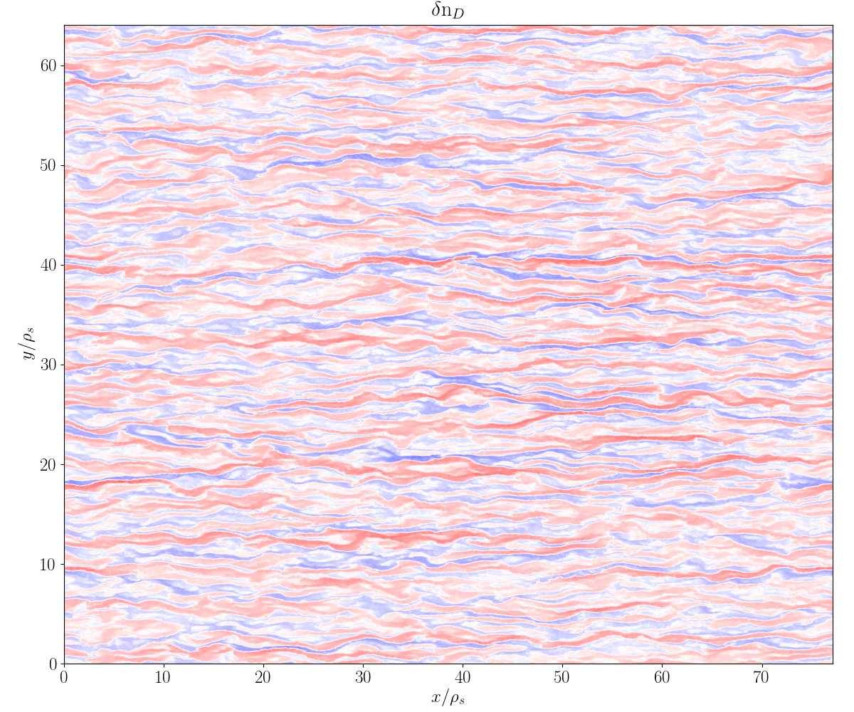
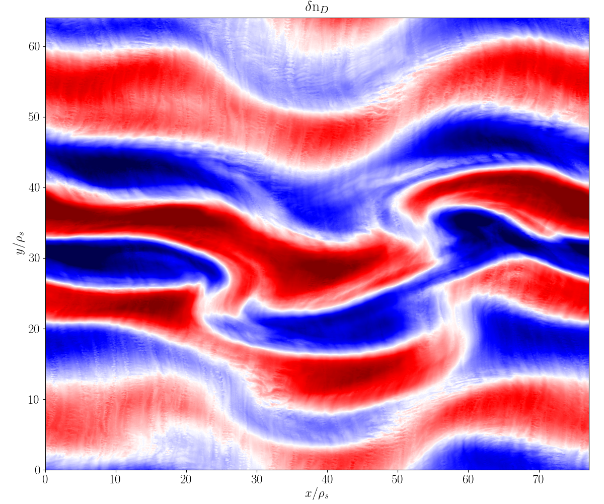
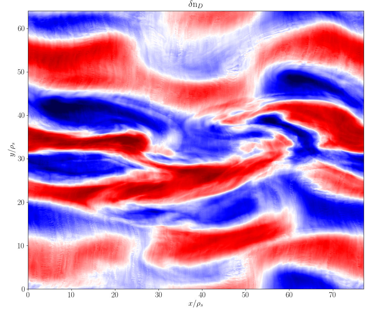
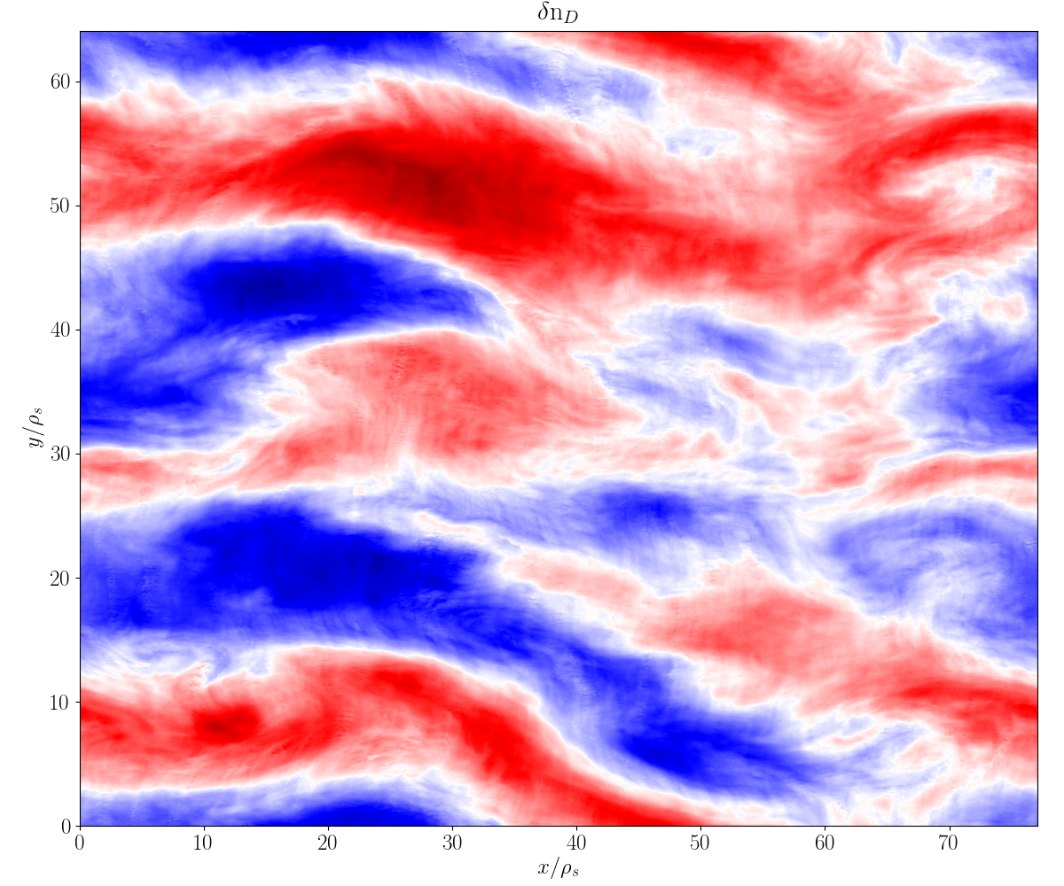
Simulation images

Simulation data courtesy Nathan Howard (MIT)

FAQ

What is $k_y \rho_s$ and why does CGYRO modify $\rho_s$ ?

The fundamental definition of the wavenumber and unit gyroradius are given in [CBB16]. These are

\[\begin{split}\begin{align} k_y \doteq &~nq/r \; , \\ \rho_s \doteq &~\rho_{s,\rm{unit}} = \frac{e B_\rm{unit}}{m_D c} \; , \\ B_\rm{unit} \doteq &~\displaystyle \frac{q}{r} \frac{\partial \psi}{\partial r} \; . \end{align}\end{split}\]

Here, $B_\rm{unit}$ is the Waltz effective magnetic field which is standard across all GACODE tools/codes, and $r$ is the midplane minor radius. For a given value of $k_y \rho_s$, the gyrokinetic equations are invariant to the scaling $n \rightarrow \alpha n$ and $\rho_s \rightarrow \rho_s/\alpha$, where $\alpha$ is an arbitrary scaling parameter.

The CGYRO input parameter KY is

\[\mathtt{KY} \doteq \Delta(k_y \rho_s) = \Delta n \left(\frac{q}{r}\right) \rho_s \; .\]

CGYRO enforces $\Delta n = 1$, which sets the (artificial) value of $\rho_s$ to

\[\rho_s \rightarrow \left(\frac{r}{q}\right) \mathtt{KY} \; .\]

To see the physical values of key parameters, you can use profiles_gen:
$ profiles_gen -i input.gacode -loc_rad 0.6
INFO: (profiles_gen) input.gacode is autodetected as GACODE.
INFO: (locpargen) Quasineutrality NOT enforced.
INFO: (locpargen) rhos/a   =+2.44577E-03
INFO: (locpargen) Te [keV] =+8.81550E-01
INFO: (locpargen) Ti [keV] =+7.58644E-01
INFO: (locpargen) Bunit    =+2.92020E+00
INFO: (locpargen) beta_*   =+4.84003E-03
INFO: ----->  n=1: ky*rhos =-7.74754E-03
INFO: (locpargen) Wrote input.*.locpargen

How does adaptive time-stepping work?

Time-stepping is controlled with the parameter DELTA_T_METHOD. Setting the parameter to 0 gives the legacy fixed timestep, whereas values greater than 0 are adaptive methods. For the adaptive methods we recommend setting DELTA_T = 0.01. Here is the recommendation:
DELTA_T_METHOD=1
DELTA_T=0.01
PRINT_STEP=100
The overall time-integration step is split between an explicit high-order step, and an implicit second-order step for collisions and trapping. When using the adaptive method, the value of DELTA_T is the size of the (large) implicit timestep. Then, the value of the explicit timestep is decreased to match the error tolerance, ERROR_TOL – the default value of which should be sufficient.

Why did you start over with CGYRO?

The past: GYRO

Over the past two decades, the fusion community has focused its modeling efforts primarily on the core region. A popular kinetic code used for this purpose was GYRO [CB10, CW03a, CW03b, CWD04]. Thousands of nonlinear simulations with GYRO have informed the fusion community’s understanding of core plasma turbulence [HHW+16, KWC05, KWC06, KWC07] and provided a transport database for the calibration of reduced transport models such as TGLF [SKW07]. GYRO was the first global electromagnetic solver, and pioneered the development of numerical algorithms for the GK equations with kinetic electrons. It is formulated in real space and like all global solvers requires ad hoc absorbing-layer boundary conditions when simulating cases with profile variation. This approach is suitable for core turbulence simulations, which cover a large radial region and are dominated by low wavenumbers.

The future: CGYRO

As the understanding of core transport has become increasingly complete, the cutting edge of research moved radially toward the pedestal region, where plasmas are characterized by larger collisionality and steeper pressure gradients that greatly modify the turbulent phenomena at play. This motivated the development, from scratch, of the CGYRO code [BC17, BC18, CBB16, CSB+19] to complement GYRO. CGYRO is an Eulerian GK solver specifically designed and optimized for collisional, electromagnetic, multiscale simulation. A key algorithmic aspect of CGYRO is the radially spectral formulation used to reduce the complicated integral gyroaveraging kernel into a multiplication in wavenumber space, but retaining the ability to treat profile variation important for edge plasmas [CB18, CBS20]. A new coordinate system that is more suitable for the highly collisional and shaped edge regime was adopted from the NEO code [BC08, BC12], which is the community standard for calculation of collisional transport in toroidal geometry.

How do you run a simple linear case?

$ cgyro -g reg08
$ cd reg08
$ cgyro -e .
$ cgyro_plot -plot ball -field 1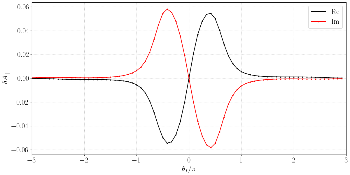

How do I run a pre-existing template case?

The input files and configuration for numerous linear and nonlinear cases can be auto-generated using the -g flag. Often, it is easiest to find a template case that is close to what you would like to run, and then modify it accordingly. A list of all regression and template cases in generated by typing:
$ cgyro -g
A very simple nonlinear case is nl00. You can generate the template with:
$ cgyro -g nl00
It is strongly suggested that you first run your case in test mode using the -t flag:
$ cgyro -t nl00
On the large systems at NERSC, ORNL and elsewhere, you will need to establish an interactive queue to execute the command above. The result should be diagnostics printed to the screen plus a few output files. Pay attention to the file out.cgyro.mpi. This shows the acceptable number of MPI tasks.

How do I submit a batch job?

On established platforms, the burden of writing batch script files and setting core counts is managed by the gacode_qsub script. To generate a batch.src file, you could type:
$ gacode_qsub -e nl01 -n 512 -nomp 2 -queue regular -repo atom -w 0:09:00
Additional flags are also accepted. Adding the -s flag to the above will submit the job.